
This post is written in R Markdown (.Rmarkdown). When you save or knit it in RStudio,
blogdown runs the R code and writes the result to index.markdown, which Hugo then turns into this page.
Summarise a data set
summary(cars)
##      speed           dist
##  Min.   : 4.0   Min.   :  2.00
##  1st Qu.:12.0   1st Qu.: 26.00
##  Median :15.0   Median : 36.00
##  Mean   :15.4   Mean   : 42.98
##  3rd Qu.:19.0   3rd Qu.: 56.00
##  Max.   :25.0   Max.   :120.00
fit <- lm(dist ~ speed, data = cars)
coef(fit)
## (Intercept)       speed
##  -17.579095    3.932409
Include a plot
plot(cars, pch = 19, col = "steelblue",
     xlab = "Speed (mph)", ylab = "Stopping distance (ft)")
abline(fit, col = "firebrick", lwd = 2)
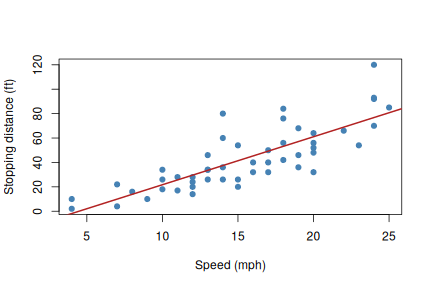
Stopping distance vs. speed
Math
Inline math like $y = \beta_0 + \beta_1 x + \varepsilon$ works, and so do display equations:
$$ \hat{\beta}_1 = \frac{\sum_i (x_i - \bar{x})(y_i - \bar{y})}{\sum_i (x_i - \bar{x})^2} $$